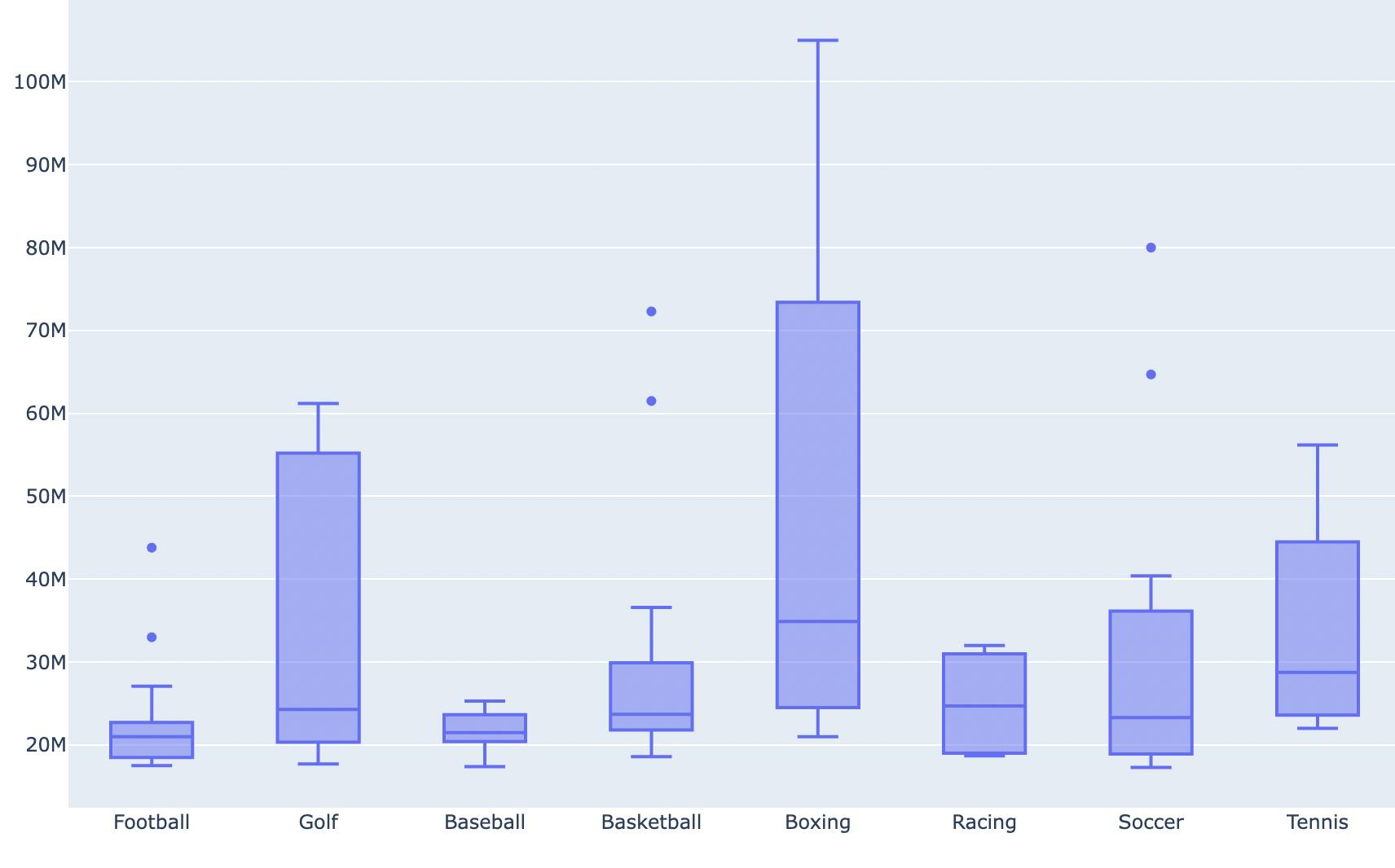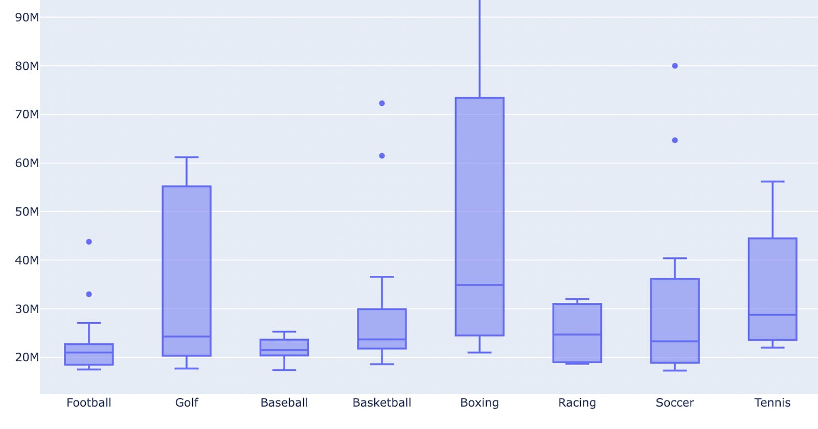
Continuing the theme of visualising data with Python, today I learned how to create boxplots with Plotly Graph Objects. Box plots visualise the variation in a dataset by representing the continuous numerical data through quartiles. They are useful for comparing two sets of data samples to each other and analysing their distributions, and they're usually used with continuous data which has a categorical feature, e.g. distribution of weight (continuous variable) by gender (category).

For practice, I used a small dataset I found on earnings of top professional athletes, and mapped the pay distribution by sports. The most interesting finding for me was that American football and baseball had the smallest variations in pay, i.e. the interquartile range (the box, which represents 50% of a category's data) wasn't huge compared to e.g. boxing where the difference between the lowest and highest quartiles was more than $50 million! Intuitively, I suspect this might be due to the "winner-takes-all" nature of the sport. The highest-paid fights are for heavyweight championship titles such as Anthony Joshua vs Oleksandr Usyk, with prize money in the millions of dollars / pounds. However, boxers that are further down the ranking or competing in lower weight categories, the prize money is much less, which might explain the large range of pay we see in this sample size.